BoxNet hasn’t seen every sample (yet). While its out-of-the-box performance is better than other unbiased and template-based methods in most cases, it probably isn’t as good as manual picking. Good news: You can teach it to be better! Here is how:

First, pick some micrographs with one of the generic BoxNets. Depending on particle density and pixel size, anywhere between 3 and 20 micrographs is a good start.

Go through the results manually in the Real Space View tab and remove False Positives or add New Particles using the mouse. When you remove a particle, it is automatically saved in a separate [Micrograph name]_[suffix]_falsepositives.star file. You can use these positions to up-weight certain areas later. If you hold Shift while removing particles, they won’t be added to the falsepositives file. When adding new particles, please make sure they are centered well. If some of the automatically picked particles are off-center, it is best to improve their positions by dragging them with the mouse instead of removing and recreating them.

Wrong labels can be tolerated to a certain degree, but the accuracy of your model will absolutely depend on the quality of the training data your provide. Try to make sure each micrograph is picked completely, since everything not labeled as a particle is labeled as background during training.

If you intend to train a BoxNet that also creates masks, it is best to already use it for the initial picking. In addition to cleaning up the particle positions, you will also have to manually paint the masks where needed.

If you clean up only a fraction of the picked items, you need to copy the corresponding STAR files to a separate folder – otherwise, all picked items will be used for training. All picking results are saved in [Input folder]/matching. It doesn’t matter where you put the separate folder, but it is convenient to make it [Input folder]/matching/training.

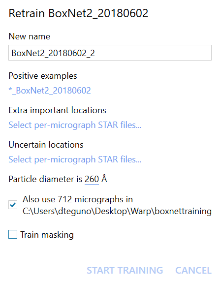
Now go to the BoxNet selection menu, select the model used for the initial picking, and click Retrain.

Give the new model a unique name. If you’re using a masking BoxNet, it’s best to keep a “Mask” in the name. Following the machine learning community’s tradition, we like to name the new models [Something]Net. Just don’t keep the name identical to the previous model, and don’t use special characters.

For the Positive Examples, select one of the cleaned up STAR files. Warp will automatically determine its suffix and match all the other files. The same goes for Extra Important and Uncertain locations. There won’t be much value in up- or down-weighting locations the first time you re-train a generic BoxNet since you don’t know yet which areas might be causing trouble. Consider using Extra Important if the first re-training doesn’t provide good results.

The Particle Diameter will determine the area around each particle’s center that is labeled as particle for training. If your sample is highly heterogeneous in size, don’t worry – this value doesn’t need to be exact.

Using the Public Data Set for re-training will dilute your new examples in a 1:1 ratio with examples contained in [Warp directory]/boxnet2training. This will prevent overfitting BoxNet on very few examples and is recommended. You may want to visit the training data repository to download the latest version.

To Train Masking, it is highly recommended to re-train a BoxNet with masking ability (i. e. one containing “Mask” in its name). Vice versa, re-training a masking BoxNet without providing masks for all training micrographs will lead to bad results. The masks will be automatically taken from [Input folder]/mask.

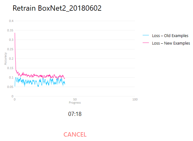
Once everything is set up, click Start Training. Warp will first prepare the new examples, load the old examples from disk (if it crashes at this point due to memory shortage, try removing some of the old examples from [Warp directory]/boxnet2training), and finally commence training.

During training, two curves (one if you don’t use the public data set) are displayed. The Loss – New Examples shows the current model’s performance on the new examples, and Loss – Old Examples shows the same model’s performance on the public data set. Over time, the loss metric for the new examples should decrease and approach that for the old examples. Meanwhile, the loss for the old examples should oscillate around the same level. It is very well possible that the loss for the new examples never reaches the old examples benchmark. This depends highly on the difficulty of your data and the quality of the labels you create (you may find the new model labels the mislabeled positions correctly, but this counts toward the loss during training). The difference between the start and end points of the new examples curve is more indicative of how much better the re-trained BoxNet model will perform on the new data.

Once the training is finished, click Close. The new model should now be listed next to the old ones, and you can select it. Test the performance on some micrographs that haven’t been used in training. If you still think it could do better, add more micrographs to the training data set and re-train again. You may also want to look into which particles the model doesn’t remember, and up-weight them during training if you think they are indeed true positives.

 

Submitting data to the public repository

Please consider contributing your training data to the public repository! Doing so will benefit all BoxNet users in the long term, hopefully bringing the out-of-the-box performance to human-like levels. You can either directly submit the data used for training your own model – it is saved as a TIFF file under [Input folder]/boxnet2training – or use the Export BoxNet Examples task dialog in the Overview tab, which has a very similar interface to the re-training dialog. Read the guidelines on the Data Upload Page and submit your training data!